Table of Contents
In the → menu, sensors can be added and basic parameters can be configured by using the Sensor Helper(see Section 5.1.2, “Sensor Helper”). After having configured the sensors, two buttons are available for each sensor: Delete and Change. These allow a user to delete or change an existing sensor with help of the Sensor Helper.
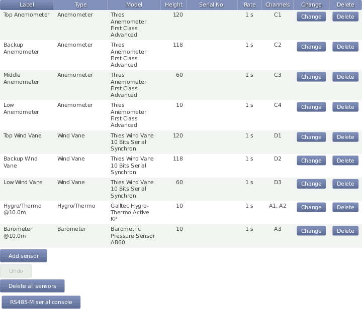
Below the sensor definitions overview you can find four buttons: Add sensor, Undo, Delete all sensors and RS485-M serial console.
- Add sensor:
Opens the Sensor Helper to configure a new sensor.
- Undo:
Click on this button to undo your last action.
- Delete all sensors
If all sensors should be deleted, e.g., after a completed measurement campaign, you can click on Delete all sensors to remove all sensors from the configuration in one step.
- RS485-M serial console
Occasionally send a command to a sensor connected to the RS485 Master port. This can be useful for debugging communication problems or to change sensor's configuration (see Section 5.1.4, “RS485 Master Serial Console”).
![[Note]](admon/note.png) | Note |
|---|---|
By clicking on a column headline in the sensor definitions overview, you can sort the selected column in ascending or descending order. |
![[Important]](admon/important.png) | Important |
|---|---|
For some estimations related to solar sensors, the GPS location of the measurement station has to be added in the → menu (see also Section 4.2, “System Administration”). |
![[Warning]](admon/warning.png) | Warning |
|---|---|
Adding or deleting a sensor, switches off recording. The new configuration is unsaved! By clicking on Switch on, recording will be activated and the configuration will be saved automatically in one step. |
To have a better understanding of the sensor management, it is important to know the difference between sensors, channels, and evaluations.
In general, a sensor is an electro-mechanical device, which records physical values. The physical values are transformed into an electrical value by the sensor. For example, wind speed can be transformed into a frequency. To map these electrical values on the corresponding physical values, an evaluation process has to be performed.
A sensor may be connected to more than one electrical channel of Meteo-40. The
number of used electrical channels depends on the kind of sensor and also on the kind of
electrical wiring of the sensor. For example, wind vane POT (potentiometer) may use the
two analog channels
A1 and
A2. Another example is the pyranometer Delta-T SN1 that emits two
analog voltage signals and one digital status signal. The two analog output signals have
to be connected to two analog voltage channels and the digital status signal has to be
connected to one digital input.
The evaluation process of the measured values is done by the software of the Meteo-40 data logger. Both pieces of data are saved: the measured physical value at every channel and the evaluated value. Some typical formulas are displayed below.
Most anemometers deliver a rectangle pulse output signal with a frequency
proportional to the instant speed. Connecting it to a counter input (i.e.,
C1 to
C12), its frequency will be measured. For the evaluation of wind speed
a linear formula will be applied using slope and offset values given in the configuration
of the
→ menu.
Equation 5.1. Linear Equation for Wind Speed
A counter value of
0 will always result in
0, i.e. the offset is ignored in this case.
The output signal of many pyranometers is an analog voltage. To measure and record
this signal, the output of the pyranometer should be connected to an analog voltage input
(i.e.,
A1 to
A12). To interpret the value of the apparent solar radiation, the
measured value is internally divided by the specific sensitivity of this sensor. In this
case sensitivity has to be configured.
In order to simplify the configuration of sensors, Meteo-40 provides a Sensor Helper in the → menu. The Sensor Helper is a wizard, which guides you through the sensor configuration. It will appear when you attempt to Add sensor or Change a sensor, a channel or an evaluation.
You must select of the available sensor types (e.g., anemometer, wind vane,
barometric pressure sensor, solar sensor, etc.) and the supported models. If the sensor
appears in the list, the appropriate channel settings will be automatically selected as
shown in
Figure 5.2, “Sensor Helper with Sensor Settings”. Depending on the sensor, further settings can be
configured by the user, e.g.,
Slope,
Offset,
Sensitivity, etc. Additionally, measurement rate, channel as well as
switch and switch pretime (if necessary) can be selected or changed.
| Important |
|---|---|
If the sensor doesn't appear in the list of preconfigured sensor, you can always use a generic sensor from the Other Sensor list. |
| Note |
|---|---|
Only channels and switches which are not already used by other sensors are available. |

| Important |
|---|---|
For many sensors, slope and offset values are pre-configured according to the manufacturer's information. Carefully check the values. If calibrated sensors are installed, use the slope and offset resp. sensitivity values indicated in the calibration protocol of the sensor. |
The order of sensors and evaluations in the web interface and the LC display is always consistent.
Sensors are ordered by
sensor type (anemometers, wind vanes, thermo/hygro sensors, barometers, precipitation sensors, solar sensors, ultrasonics, power meters, other sensors),
height (from highest to lowest),
and finally the textual label (alphabetically).
Evaluations are ordered by
evaluation type (wind speed, wind direction, humidity, temperature, differential temperature, air pressure, air density, etc.)
height of the corresponding sensor (from highest to lowest),
and finally the textual label (alphabetically).
During the installation process or in case of communication problems, it can be useful to send a special command to a connected RS485 sensor.
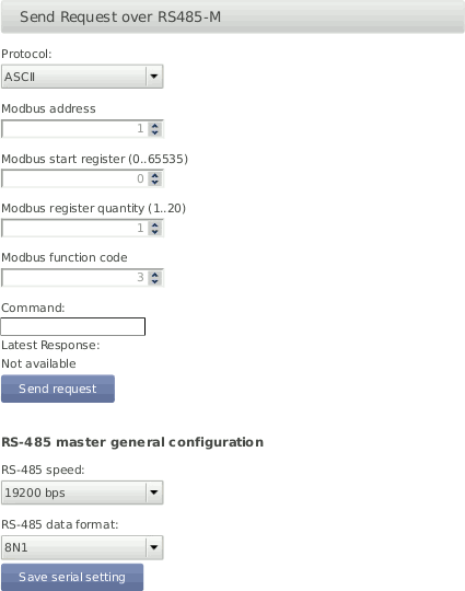
First of all, the RS485 Master general serial settings must be set matching sensor's configuration. These settings affect not only the serial console but any other RS485 sensor configured.
If Modbus protocol is selected, the telegram will be internally composed, according to the selected address, start register (PDU addressing, first reerence is 0), register quantity and function code, and shown in the command box. If ASCII protocol is selected, the command must be typed by the user in the command box. The following escape sequences representations are recognized for the ASCII commands:
Table 5.1. ASCII escape sequences for RS485-M serial console
| Escape Sequence | Symbol |
|---|---|
| <CR> | \x0d |
| <LF> | \x0a |
| <STX> | \x02 |
| <ETX> | \x03 |
The communication will be reflected in the logbookincluding a timestamp. Example of ASCII communication: "RS485-M Request: '01TR00003<CR>', Response: '<STX>000.1 096 +24.6 M 0E*1D<CR><ETX>'". Example of Modbus communication: "RS485-M Request: '0104277400063aa6', Response: '01040c41375c2942c0000041e800006d3d'".
| Note |
|---|---|
The RS485-M serial console is only available for Admin. |
In the → menu a table is shown, which displays all connected channels with details such as label, value, rate, range, protocol and selected switch. To modify sensor settings, click on Change to start the Sensor Helper(see also Section 5.1.2, “Sensor Helper”).
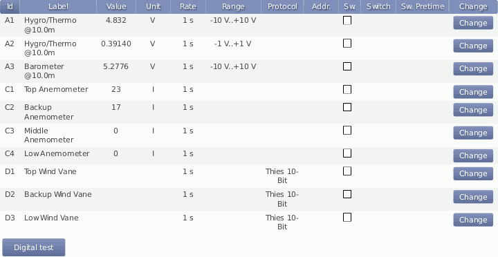
| Note |
|---|---|
Click on a column headline in the measurement channels overview to sort the selected column in ascending or descending order. |
In the → menu the settings for data evaluation are shown. A table displays the configured sensors with their measured and estimated values. The order of evaluations is explained in Section 5.1.3, “Order of Sensors and Evaluations”. If the settings should be modified, click on Change to start the Sensor Helper(see also Section 5.1.2, “Sensor Helper”).

In addition to the automatically generated evaluations, it is possible to apply formulas to the measured values or even combine evaluations. The new evaluations can be added in the Evaluation Helper by clicking on Add evaluation. See Section 5.3.1, “Evaluation Helper”.
| Note |
|---|---|
Click on a column headline in the evaluation configuration overview to sort the selected column in ascending or descending order. |
The Evaluation Helper introduces a higher flexibility to Meteo-40 sensors configuration. A part from the automatically configured evaluations which appear when you add a sensor, this tool allows you to generate new evaluations, combining the existing by means of a formula. The standard statistics will be available for this new evaluation and will be included in the CSV statistics file. The Evaluation Helper also provides some special statistics like the covariance, kurtosis, turbulence intensity or Obukhov length. To use this feature, click Add evaluation in the → menu. The Evaluation Helper will guide you through the configuration process. After choosing a formula from the list, the corresponding parameters will be shown for selection.
| Important |
|---|---|
Only the measured values are saved by default to the CSV statistics file. Estimated values are for information purposes. In order to include estimated values in the CSV statistics file, select the values over the statistics selection interface in the → menu under Select statistics(see also Section 6.3.1, “Configuring Statistics and CSV files”). |
Surface albedo is defined as the ratio of irradiance reflected to the irradiance received by a surface. It is dimensionless and measured on a scale from 0 (corresponding to a black body that absorbs all incident radiation) to 1 (corresponding to a body that reflects all incident radiation).
Based on the Ohm's law, you can use the Ampere meter formula to transform the measured voltage to the corresponding current, after introducing the value of the shunt resistor used. This formula can be used with any existing voltage evaluation (e.g. if you previously configured a Gantner A3.1 module).
(where I is the current through the conductor in units of amperes, V is the voltage measured across the conductor in units of volts, and R is the resistance of the conductor in units of ohms)
According to IEC 61400-12-1 it is required to measure air density, which is calculated from air temperature and air pressure. Air density has a significant influence on the wind energy calculation. See calculation of wind energy in Section 10.1, “Sensors for Wind Resource Assessment and Wind Farm Monitoring”.
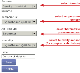
At high temperatures measuring relative air humidity is recommended according to IEC 61400-12-1. In order to calculated density of moist air, Meteo-40 offers two options: with or without relative humidity.
If air density should be calculated without humidity, choose only a temperature and a barometric pressure sensor from the list in the Evaluation Helper. Meteo-40 calculates air density for evaluation with original 1-sec measurement data according to the following formula:
(where p is the air pressure, T the air temperature and R O the gas constant of dry air 287,05[J/kgK])
If relative humidity should be considered for air density calculation, choose also a humidity sensor from the list in the Evaluation Helper. With selected humidity sensor, Meteo-40 calculates density of moist air for evaluation with original 1-sec measurement data according to the following formula:
Equation 5.7. Calculation of Density [ρ] of Moist Air
(where T is the air temperature, p the air pressure, R 0 the gas constant of dry air 287,05[J/kgK], R H 2 O the gas constant of water vapour 461,5[J/kgK], p H 2 O the vapor pressure, RH the relative humidity)
The dew point is the temperature to which air must be cooled to become saturated with water vapor. If the temperature (T) and relative humidity (f) are measured, it is possible to calculate the Dew point configuring it in the Evaluation Helper. The following formula is applied.
(where T is the measured temperature and f is the measured relative humidity)
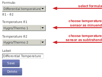
By selecting Differential temperature in the Evaluation Helper, the difference between two temperature measurements can be recorded every second. Choose two temperature sensors from the list for theta 1 and theta 2. According to the following equation the difference is calculated.
Incoming long wave irradiance received from the atmosphere. Pyrgeometer equation by Albrecht and Cox.
(where Ein is the ong-wave irradiance received from the atmosphere [W/m²], Enet is the net irradiance at sensor surface [W/m²], σ is the Stefan–Boltzmann constant 5.670374419 x 10^-8 [W/(m^2·K^4)] and T is the Absolute temperature of pyrgeometer detector [K]
Angle off the horizontal plane at which the wind flow comes into the sensor.
(where V z is the vertical wind speed and V h is the horizontal wind speed)
The linear equation can be used with any existing evaluation in order to apply an slope and offset. It can also be used to provide a dimensionless measurement (e.g. from a previously configured Other sensor) with a unit and an evaluation type for better interpretation.
The Obukhov Length can be useful for turbulences analysis and is typically associated with a 3D ultrasonic sensor. To add this evaluation, the measurement of wind speed, wind direction, vertical wind speed and virtual temperature at one height are needed.
(where u * is the friction velocity [m/s], g the graviatitonal acceleration 9.81[m/s²], σ(V Z,T) the covariance of vertical wind speed and virtual temperature and K the von Kármán constant 0,41)
Dimensionless stability parameter given by the normalized measuring height above ground z with the Obukhov length L. Can be useful for turbulences analysis and is typically associated with a 3D ultrasonic sensor. To add this evaluation, the measurement of wind speed, wind direction, vertical wind speed and virtual temperature at one height are needed.
(where z is the height above ground and L is te Obukhov length as in Section 5.3.1.12, “Obukhov length”)
Sensible heat flux measured with the eddy covariance method. In meteorology, the conductive heat flux from the Earth's surface to the atmosphere.
(where ρ is the air density 1.2[kg/m 3], C p the specific heat with constant pressure 1004.67[J/K/kg] and σ(V Z,T) the covariance between the vertical wind speed and the temperature)
The solar zenith angle is the angle between the zenith and the centre of the Sun's disc. It is calculated from the configured latitude and longitued and the time in the moment of the calculation.